It is quite common in most workplace situations to find the need to add additional Rows or additional Columns to the Source Data File that is being used by a Pivot Table.
In such cases, you can correct the Pivot Table by changing its “Data Range” to include the newly added columns and rows in the Source Data File.
However, if the Source Data arrives in a new worksheet, you will find the need to change Pivot Table Data Source from old to New Spreadsheet.
1. Change Pivot Table Data Range
When new Rows or Columns are added to the Source Data File, you can follow the steps below to change the Data Range for your Pivot Table.
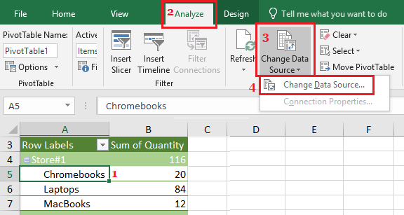
1. Click on any Cell in the Pivot Table and this will bring up “Analyze” and “Design” Tabs in the top menu bar.
2. Next, click on Analyze tab > Change Data Source > Change Data Source… option in the drop-down menu.
3. In Change Pivot Table Data Source dialogue box that appears, click in Table/Range box and select the entire Data Range (including new Rows & Columns) that you want to include.
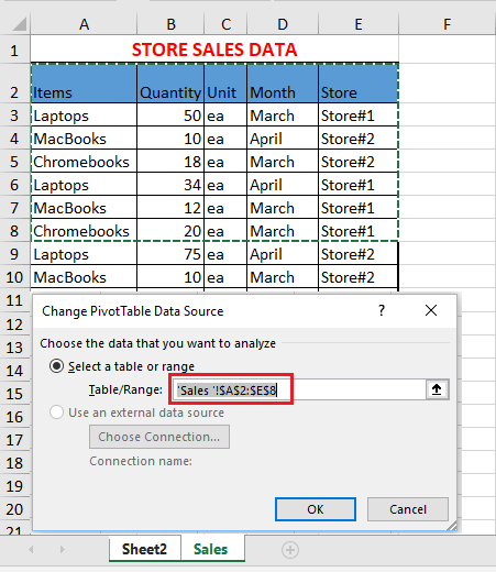
3. Click on OK to save the changes.
2. Change Pivot Table Data Source Worksheet
If the Source Data for Pivot Table has arrived in the form of a new worksheet, you will be required to change the “Data Source” for your Pivot Table.
1. Click on any Cell in the Pivot Table and this will bring up “Design” and “Analyze” tabs in the top menu bar.
2. Click on Analyze > Change Data Source > Change Data Source option in the drop-down menu.
3. In Pivot Table Data Source dialogue box that appears, click in Table/Range box and click on the Worksheet containing new Source Data.
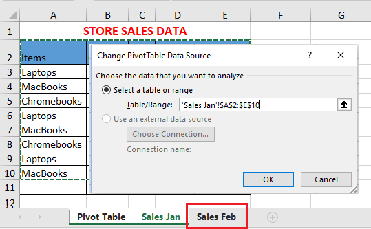
As you can see in above image, the “Table/Range” field refers to “Sales Jan” worksheet and clicking on “Sales Feb” will change Data Source for Pivot Table to the new worksheet.
After changing Data Source, make sure that Data Range includes all the rows and columns that need to be incorporated in the Pivot Table.
4. Click on OK to save the changes.