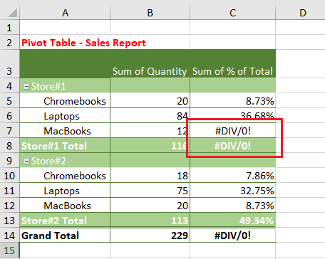
When you make use of Formulas or calculations in an Excel Pivot Table, the Pivot Table is likely to come out with some Empty Cells and Cells with #DIV/0! Error values.
As you may agree, such errors do not look good in a Pivot Table and can raise questions, both when you submit the Pivot Table as a part of your report and also while you are using the Pivot Table in an online or live presentation.
Fix Error Values in Pivot Table
If the reason for #DIV/0! Error values in a Pivot Table is due to a number being divided by zero, this can be easily fixed by making Microsoft Excel replace such Error Values by a Custom defined value or Text.
However, #DIV/0! and other types of error values in a Pivot Table can also be caused due to calculation errors and Incorrect formulas in the Data Source File being used by the Pivot Table.
Hence, it is really important that you thoroughly check and make sure that there are no incorrect Formulas or calculation errors in the Source Data File, which is being used by the Pivot Table.
If you are completely satisfied with the correctness of Formulas and calculations in Source Data File, you can follow the steps below to fix #DIV/0! error in Pivot Table (if they are still there).
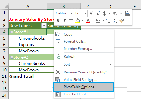
1. Fix #DIV/0! Error in Pivot Table
1. Right-click on the Pivot Table and click on PivotTable Options in the drop-down menu.
2. On PivotTable options screen, check the little box next to For error value show: and enter NA (Not Applicable) or any other text that you want to show up in the Pivot Table in place of the Error Value.
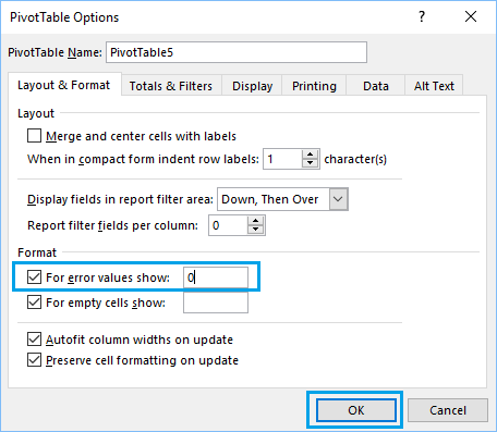
3. Click on the OK button to save this setting in the workbook.
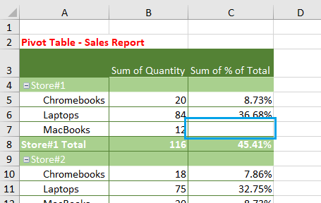
Now, whenever the Pivot Table comes across #DIV/0! error in the source data file, it will be automatically replaced by NA (Not Applicable).
Important: A drawback of this solution is that it can mask future errors in source data file. Hence, always make sure that formulas and calculations in source data file are correct and free from errors.
2. Fix Empty Cells in Pivot Table
Whenever the Source Data File for a Pivot Table contains blanks (which usually happens), you may see empty or no values in certain cells of the Pivot Table.
Just like other errors, empty values in a Pivot Table do not look good and they can also lead to waste of time due to questions about them during your presentation.
1. Right-click on the Pivot Table and click on PivotTable Options in the drop-down menu.
2. On PivotTable options screen, check the little box next to For empty cells show: and enter “O” or “NA” in the box.
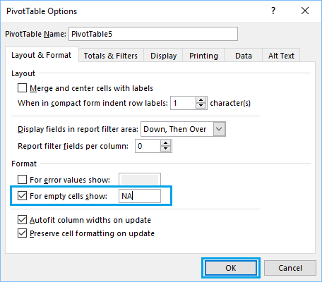
3. Click on OK to save this setting.
Now, all the empty values in your Pivot Table will be reported as “0” which makes more sense and is more acceptable than seeing blanks or no values.
3. Fix “Blank” Value in Pivot Table
Sometimes, you may find the Empty Cells in a Pivot Table being reported as “blank”, which also can raise questions about the correctness of the Pivot Table.
As mentioned above, the reason for this error is due to presence of Empty cells in the Source or Data File being used by the Pivot Table.
You can either fix this error by using Custom Values (methods as discussed above) or hide “blank” in Pivot Table by following these steps.
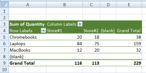
1. Identify the Location of “blank” values in the Pivot Table. In this case, the word “blank” is appearing in Row 8 and also in Column C of the Pivot Table.
2. Click on the Down-arrow located next to “Row Labels” and uncheck the little box located next to blank and click on the OK button.
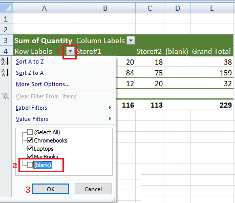
This should result in all the “blank” values in the Pivot Table being hidden.