If you are usually working with large worksheets, it is really important that you become familiar with the steps to Freeze Rows and Columns in Microsoft Excel.
For example, if the spreadsheet has “Column headings”, Freezing the top-row containing Column headings can prevent the Column headings from going out of the view, when you scroll down the worksheet.
Similarly, if the worksheet spans across multiple columns you may find the need to make a particular column or columns remain visible, when you scroll to the side on the worksheet (Right or Left).
Freeze Rows and Columns in Excel
The exact function that allows you to Freeze Rows and Columns in Microsoft Excel is known as “Freeze Panes” and it is located in the View Tab of the top-menu bar in Microsoft Excel.
You can find below the steps to Freeze Rows, Freeze Columns and Freeze both Rows & Columns using the “Freeze Panes” function in Microsoft Worksheet.
Note: Freezing Rows or Columns has no effect on printing, it only affects the way that worksheet appears on the screen.
1. Freeze Rows in Excel
Perhaps the most commonly used application of Freeze panes function in Microsoft Excel is to Freeze the Top-row containing Column Headings.
This ensures that the Column Headings always remain visible when you scroll down the Worksheet, which makes it easy review existing data and enter or modify data in the right columns.
1. Select the Row (or the first cell in the row) right below the Top-row which contains the Column headings.
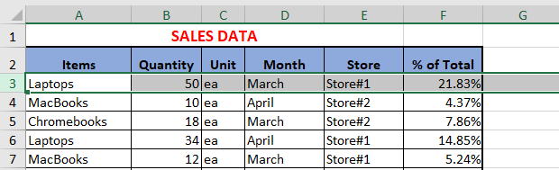
2. Next, click on the View tab > click on Freeze Panes and then click on Freeze Panes option in the drop-down menu.
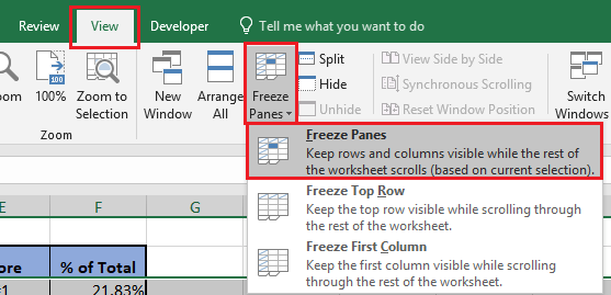
This will freeze the Row containing Column Headings and this particular Row will always stay visible when you scroll down the worksheet.
2. Freeze Columns in Excel
If the worksheet spans multiple columns you can make a certain column or columns always visible when you scroll to the side on the worksheet (Right or Left).
1. Select any Cell located immediately to right of the Column that you want to freeze. In our case, we have selected Cell B2, in order to Freeze Column A containing “Items”.
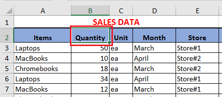
2. Next, click on the View tab > click on Freeze Panes and then click on Freeze Panes in the drop-down menu.
This will Freeze Column A and this particular Column will always stay visible when you scroll sideways on the worksheet
3. Freeze Both Rows and Columns in Excel
In certain cases, you may want to Freeze the Row containing Column Headings and also Freeze the first column or few selected columns in the worksheet.
To Freeze both rows and columns, select the Cell located to right of the Column that you want to Freeze and below the Row that you want to Freeze.
In our case, we have selected Cell B2 in order to Freeze the second Row containing column headings and also Freeze Column A containing “Items”.
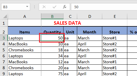
After selecting the right-cell, click on the View tab > Freeze Panes > Freeze Panes option in the drop-down menu.
Now the rows above the selected Cell will remain frozen when you scroll down and also the Columns to the left of the selected Cell will also remain frozen when you scroll to the side.
Unfreeze Rows and Columns in Excel
At any time, you can Unfreeze Rows and Columns in Excel by clicking on the View Tab > Freeze Panes > Unfreeze Panes option in the drop-down menu.
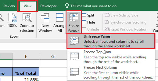
The Frozen Rows or Columns will become free and they will no longer remain frozen or stationary when you scrolled up or down.
Freeze Panes Not Available in Excel
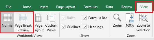
You may come across an issue where the Freeze Panes option is not available, appears grayed out or it does not work. This problem is usually related to the worksheet being in “Page Layout” view.
To fix this issue, click on the View Tab and then click on Normal or Page Break Preview.
In certain cases, the Freeze Panes option can also get disabled due to the workbook being in protected mode.
However, this issue has been fixed in the newer versions of Microsoft Excel and you may face this problem, only while working on files created using an older versions of Excel (older than Excel 2013).