The SUMIF function in Microsoft Excel can be used to Count the total number of items in a list, only when they match a specified criteria or condition.
For example, the SUMIF Function can be used to instantly find the total number of only the Apples sold at a store from a combined list of Apples, Oranges and Mangoes sold at that particular store.
Instead of manually going through the long list of items to identify and count similar items, you can use the SUMIF Function to do this job for you in a very short time.
Use SUMIF Function in Excel
The SUMIF Function in Microsoft Excel is written in the following format.
=SUMIF(range, criteria, [sum_range])
Range: The range of cells on which you want to employ the criteria.
Criteria: The criteria determining which cells to Add.
Sum_range: The range of cells within which the numbers meeting the Criteria are located.
Steps to Use SUMIF Function in Excel
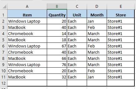
In order to understand the use of SUMIF Function in Excel, you can consider the following sales data providing the number of Windows Laptops, MacBooks and ChromeBooks sold at Store#1.
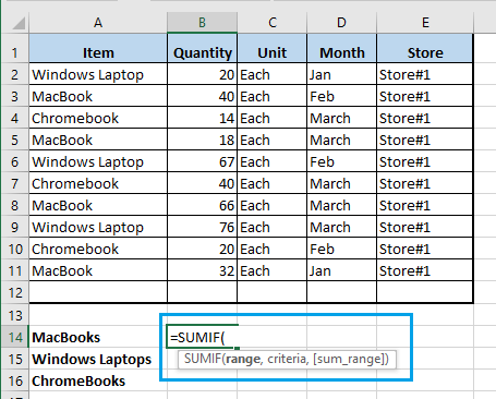
Now, the task is to find only the total number of ‘MacBooks’ sold using the Excel SUMIF Function.
1. Place the cursor in Cell B14 and start typing =SUMIF and Microsoft Excel will automatically provide you with the Syntax to follow (=SUMIF(range, criteria, [sum_range]).
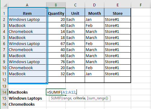
2. Going by the Syntax provided, first select Cells A1:A12 as the Range – This is where the item (MacBook) that you want to count is located.
3. Next, specify the Criteria by clicking on Cell A3 – As this Cell contains the name of item (MacBook) that you want to Sum.
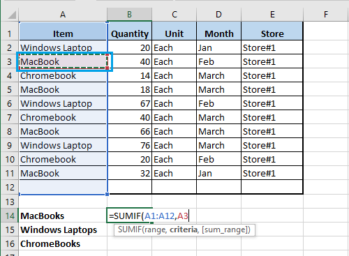
Note: You can also click on any cell containing the term MacBook (A5, A8, A11)
4. Select Cells B1:B12 as the sum_range – This is where the count for number of items (MacBook) sold is located.
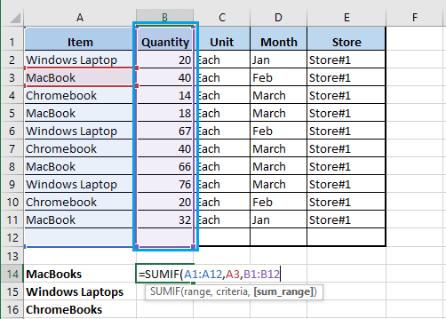
5. Finally, close the bracket and press the Enter Key.
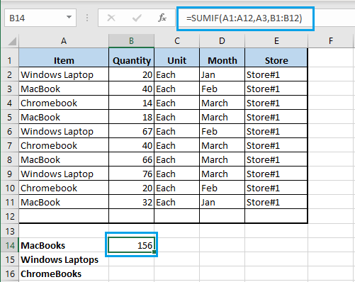
The SUMIF formula will instantly display the total number of MacBooks sold at the two store locations.
Similarly, you can use the SUMIF Function to count the total number of Windows Laptops and ChromeBooks sold at the two store locations.