In case you do not want a certain value or values appearing in Pivot Table, you can hide them. In this tutorial, you will find the steps to hide and unhide values in Pivot Table.

Hide Values in Pivot Table
Follow the steps below to Hide Values in Pivot Table.
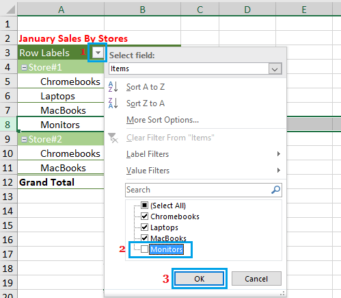
1. First, identify the Items or Values that you want to hide in Pivot Table. In our case, we are going to hide the Value located in Row Number 8 under Column A.
2. Next, click on the Down Arrow located to the right of the Label under which the item or value that you want to hide is located.

3. In the Drop-down, unselect the checkbox next to the Item or Value that you want to hide and click on OK to save this setting. In our case, we are hiding the item “Monitors” by unchecking this item.
Now, when you view the Pivot Table, you won’t be able to see the Value or Item that you had unchecked.
Unhide Values in Pivot Table
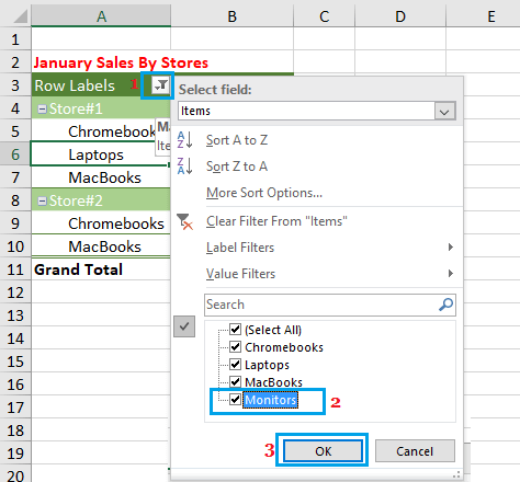
Whenever a Pivot Table contains a hidden value or values, you will see a Filter Icon next to the Column Label containing the hidden value, which makes it easy to identify the location of hidden values.
To Unhide Values in Pivot Table, click on the Filter icon next to the Label under which the values are hidden. In the drop-down menu, select the check box next to the Hidden Value/Values and click on OK.

In our case, we have selected the checkbox next to item “Monitors’ in order to unhide and show this item in our Pivot Table.
Once you Unhide Items or Values in Pivot Table, you will no longer see the “Filter icon” next to the Column heading under which the values were previously hidden.